Act 6 Preparation

Back in activity 2, we used scilab to look at the Fourier Transform(FT) of simple geometric shapes. In this preparatory activity, we're going to do that again, albeit with the addition of dimensionality, rotation, and translation.


Coding part step-by-step (REALLY!)  (code given by Dr. Soriano, might be edited a little)
The grid is set up

x = [-2:0.05:2];
y = [-2:0.05:2];
[X,Y] = meshgrid (x,y);
r = sqrt(X.^2 + Y.^2);

 x and y become arrays from -2.0 to 2.0 in steps of 0.05, i.e. [-2.,-1.95,-1.90, ... -0.05,0,0.05,... 1.90,1.95,2.00]
[X,Y] is the 2D array which we can think of as one similar to the xy coordinate system. X is x repeated 81 times, Y is basically X transposed.
r is the distance from the center to a point in [X,Y]

A 2D array filled with zeros represents a black 81x81 image.

m = zeros(size(x), size(y))

Some parts of it are selected to become nonzero; 1.0 is chosen since that value corresponds to white in scilab bw images.

m(find(r<0.5)) = 1.0;

From the inside-out, in baby steps:

• if we declare an integer j = 0.25 and we type j < 0.5, scilab returns "T" since x is less than 0.5
• if j is instead, an array, scilab evaluates each element of the array and returns an identically size array of the same size. i.e. if j = [0.25,0.5,0.75], j<0.5 returns [T,F,F]
• r<0.5 therefore gives us all the points in XY within a circle of radius 0.5
• find(r<0.5) gives the indices of r which are true
• m(find(r<0.5)) identifies all elements of m whose mirror in r<0.5 is 
• m(find(r<0.5)) = 1.0 sets all aforementioned elements to 1.0

m can now be displayed in 3D
imesh(m);
or topview
imshow(m);

<1>
caption
Matrix m displayed in (left)3D and (right)topview


A few coding notes:
In the code given to us,
grayplot(x,y,(FTmc)) was used to show the topview of the FT. According to the documentation, 

grayplot makes a 2D plot of the surface given by z on a grid defined by x and y. Each rectangle on the grid is filled with a gray or color level depending on the average value of z on the corners of the rectangle.

Apparently, grayplot smoothens the image, leading to a loss of detail. That's why I chose to use imshow for the real space images. However, the regular imshow gets cranky with the images in frequency space, you need to specify the colormap to make it presentable. imshow(FTimage, hotcolormap(8)) works for my FT-ed images. :) HOWEVER, all the pictures here are in grayplot, since I always mess things up when doing repetitive actions.


mfft(m,-1,[81 81]) was used to take the FT of the image. It's a multidimensional FT, you just have to specify the matrix, flag( -1  denotes FT, 1 denotes inverse FT), and dimensionality(our matrix is 81 by 81). An alternative is using fft2(m) for the 2D FT and ifft(m) for the inverse FT.


Necessary pics


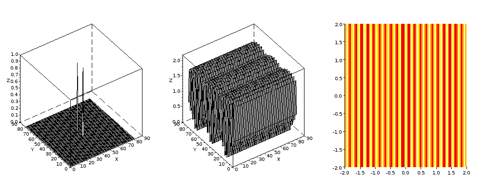
The pics are ordered with the original shape at the left, the FT in the middle, and the topview of the FT at the right.

Dirac deltas symmetric with respect to the y axis. The distance from the y axis is increased from 5 to 30.

Cylinders with (top to mid) distance from the y axis increased from 5 to 20 and (mid to bot) radius increased from 2 to 10

Gaussian functions of various variances along the x and y.

 

Squares (top to middle) displaced and (middle to bottom) increased in size

entire code:
mtlb_close all;
// CREATE A MATRIX OF X AND Y COORDINATES WITH
// THE ORIGIN AT THE CENTER

x = [-2:0.05:2];
y = [-2:0.05:2];
[X,Y] = meshgrid (x,y);
R = sqrt(X.^2 + Y.^2);

// INITIALIZE A CLEAN MATRIX
m = zeros(size(x), size(y));

//point sources at distance d from the y axis
//d = 5;
//m(41+d,41)= 1;
//m(41-d,41) = 1;

//circles of radius r at distance d from the y axis
//r = 10
//d = 20
//m(find(R<0.2)) = 1.0;
//m = [m(:,1+d:40+d), m(:,41-d:81-d)];

//squares of length l at distance d from the y axis
//l = 0.5
//d = 20
//m(find((abs(X) <=l)& (abs(Y)<=l)))=1;
//m = [m(:,1+d:40+d), m(:,41-d:81-d)];

//gaussian of variance var
varx = 0.1;
vary = 0.05;
m = exp(-(X.^2)/varx-(Y.^2)/vary);

FT = mfft(m,-1,[81 81]);
FTmc = fftshift(abs(FT));

a = scf(1);
xset("colormap", hotcolormap(128));
subplot(131);
mesh(m);
subplot(132);
mesh(FTmc);
subplot(133);
grayplot(x,y,(FTmc));
a.figure_size = [1000,500];
xs2png(a, "Documents/AP186/act 6/CMap gauss varx0.1 vary0.05.png");