Act 4: Area estimation

Last month, I ran around the Louvre for 3 hours and barely made a dent in the amount of things to see. Since I get a little claustrophobic when I'm surrounded by a lot of people during my "paying attention" mode, I strode past Mona Lisa, Venus de Milo, and all of the popular ones and soaked in the rooms of exhibits that were left unadmired. Even though I didn't understand a drop of French, it was all quite fascinating, really. I can imagine staying inside for days, just tracing the outlines of statues with my eyes and wondering about the history of tiny trinkets.

Anyway, today, we will take this screenshot of the Louvre(from google maps) and use digital methods to approximate its area.

Figure 1. Screenshot of the Louvre from Google maps

How do we do this? Well, notice that little map scale in the lower left corner? We're going to use it. ;)

In this screenshot, it takes 64 pixels to span 100 meters, thus we can equate 1 pixel to 100/64 meters per dimension. Next, we need to find the number of pixels covered by the Louvre, then, multiply it by the square of (100/64) to get the actual area covered by the grounds of the Louvre. Simple, right? Everybody knows how to count! ... but since this is roughly 1600x1000, it's just not that practical to count it by hand. :/
Thus, we make the machine count!

First, we make the map "machine readable" by coloring in the area of the Louvre.

Figure 2. Area of the Louvre in white

Instead of making the machine count the number of white pixels, an alternate way to get the area is by inferring the area(or volume) by integrating over the perimeter(or surface). This is called Green's theorem. For our purposes, it's the same as dividing the area into triangles, and by knowledge of the vertices, add their areas up together. This is exemplified in the formula:

where x and y are the pixel locations of the vertices.

The implementation looks like this:

Img = imread('Documents/AP186/act 4/louvre.bmp');Img = im2bw(Img, 0.8);  //converts image into black and white, so that white = 1, black = 0

pixelCount = size(find(Img)); //pixel counting method

greensThm = 0;[x,y] = follow(Img);  //picks out the vertices
for i = 1:length(x)-1  greensThm = greensThm + x(i)*y(i+1) - x(i+1)*y(i);   //using the formula derived from Green's theorem 
endgreensThm = 0.5*greensThm;

Testing out different shapes, we get the following values, with "error" obtained with the number obtained through pixel counting defined as the correct value.

Table 1. Comparison of pixel counting method and Green's theorem

	square	triangle	pentagon	circle	louvre
Green's theorem	8953	9447.5	8947	7733.5	175474.5
pixel counting	9216	9676	9162	7908	176481
error	2.9%	2.4%	2.4%	2.3%	0.5%

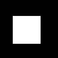
In the case of the square, one can observe that 9216 is equal to the square to 96, while 8953 is between the square of 94(8836) and 95(9025). Perhaps this can be attributed to the contour not being included in the evaluation. Although this is a big problem for small images, the error will decrease as the resolution increases(if the object is a mostly solid shape). For our purposes, we will disregard this.

Figure 3. Images used for comparison

Getting back to the original problem, the Louvre has 176481 pixels. Multiplying it twice by 100/64, we get 430,861 square meters. By reading tourist pamphlets, we know that the Louvre has an area of approximately 40 hectares or 400,000 square meters! Taking that as the true value, simple pixel counting leads to a discrepancy of 7.7%, which could be easily accounted for by overestimation of the official grounds of the Louvre or exclusion of half of the pixels in the tick marks in the map scale.


For this activity, I will give myself a grade of 9. Although I was able to get the desired results with reasonable accuracy, I did not fully appreciate the use of Green's theorem, as I feel that a simple sum(image array) in python will produce the desired result more efficiently.