Act 6. Repetitive? Image Manipulation in Frequency Space

In this activity, we will edit images in ... dundundun... frequency space!

Instead of

normal picture > edit > finished picture

we will do
normal picture > (Fourier Transform - transfer to frequency space) >  edit > (Inverse Fourier Transform - leave frequency space) > finished picture

The Fourier Transform looks for patterns in the image. Each point in frequency space represents a sinusoidal pattern, with the persistence of that pattern as the amplitude at that point. Edges (or a rapid change in intensity) in an image which do not repeat periodically are represented by low frequency values. Smooth areas with a little bit of noise varying across it seem to repeat with a high frequency. These types of filters are pretty easy to implement, we just have to use m(find(r>0.5)) for a high pass filter, replace the > with a < for a low pass filter, and combine them for a band pass filter.


The following images are arranged according to (top) image, (bottom)frequency space, (left)original image, (middle) filtered components, (right) resulting image.

High pass filters. It can be used to smoothen edges. Try using a highpass filter on your picture - your pores will disappear!

Low pass filter. Can grab edges. The resulting photo now emphasizes the changes in the  original image.

Band pass filter. I'm not really sure how this is normally used, but it was able to (coincidentally) grab the weave of the painting (middle).

The task for this activity is to remove repeating patterns from images.

Specifically, the horizontal lines from

Lunar orbiter image with lines

and the weave from this painting.

Painting by ___ with a noticeable weave pattern

The methodology used is

1. Go to the frequency space in Scilab.
2. Save the FT
3. Open the FT in an image editing program(Gimp).
4. Create a white layer on top.
5. Add black/gray dots on top of the high amplitude points in the FT (you have to lower the opacity of the blank layer).
6. Save.
7. Open it up in Scilab
8. Multiply the filter with the FT of the original image.
9. Take the inverse FT.
10. You have your finished image. :D

But since my Gimp kept on crashing :( I decided to do it purely in Scilab instead.

I took a look at the histogram of the natural logarithm of the FT amplitudes.

(histplot of log(FT))

I took an arbitrary mark that I estimated would include the bright spots in the FT. I then added a criterion that would isolate the general area where I expect the FT of the undesired repeating pattern. A circle around the center was left as is because changing it would remove important details from the image. I replaced these areas with 10, and not with 0, because it was just below the median value.

Deletion of lines from the lunar orbit picture (left) original (middle) extracted (right) resulting image

Code for the lunar picture

moon = gray_imread("Documents/AP186/act 6/crater.jpg");
x = [-0.5:1.0 / (size(moon,1)-1):0.5];
y = [-0.5:1.0 / (size(moon,2)-1):0.5];
[X,Y] = meshgrid(y,x);
r = sqrt(X.^2 + Y.^2);
moonF = fftshift(mfft(moon,-1,[size(moon,1),size(moon,2)]));
a = scf(1);
subplot(231); //original image
imshow(moon);
subplot(234); //FT original image
imshow(log(abs(moonF)),bonecolormap(8));
subplot(235); // filtered out (frequency space)
erased = ones(size(moonF,1), size(moonF,2));
erased(find(log(abs(moonF)) > 4  & abs(X)<0.01 & r > 0.015)) = moonF(find(log(abs(moonF)) > 4 & abs(X)<0.01 & r > 0.015));
imshow(log(abs(erased)),bonecolormap(8));
subplot(232); // filtered out (real space)
imshow(mfft(erased,1,[size(moon,1),size(moon,2)]));
subplot(236); // edited image FT
moonF(find(log(abs(moonF)) > 4 & abs(X)<0.01 & r > 0.015)) = 10.0;
imshow(log(abs(moonF)),bonecolormap(8));
subplot(233); //edited image
moonFix = mfft(moonF,1,[size(moonF,1),size(moonF,2)]);
imshow(abs(moonFix),bonecolormap(8));
a.figure_size = [1000,800];
xs2png(a, "Documents/AP186/act 6/moonsir cool.png");

A similar code was used for the painting, but the criterion for masking in the frequency space was instead

find(log(abs(snipF))>4 & r > 0.1)

Extraction of weave from painting  (left) original (middle) extracted (right) resulting image

By blowing up the top left and top middle pictures, we can see that a general approximation of the triangularly shaped weave is obtained.

(Left) Original texture and (right) extracted texture

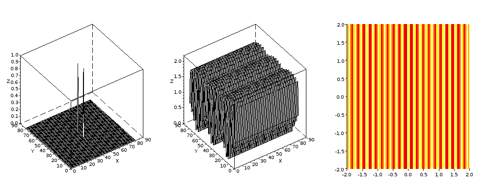
Part of the preparation for this activity was looking at the convolution(or multiplication in frequency space) of two images of dissimlar sizes. It is supposed to used as familiarization with applying filters. 

(Left) Ten random points (middle) convolved with a 5x5 image (right) points in a periodic fashion

I would give myself a grade of 11 for being able to get the desired output (lunar picture without lines and painting without weave) without using external applications.

Act 6 Preparation

Back in activity 2, we used scilab to look at the Fourier Transform(FT) of simple geometric shapes. In this preparatory activity, we're going to do that again, albeit with the addition of dimensionality, rotation, and translation.


Coding part step-by-step (REALLY!)  (code given by Dr. Soriano, might be edited a little)
The grid is set up

x = [-2:0.05:2];
y = [-2:0.05:2];
[X,Y] = meshgrid (x,y);
r = sqrt(X.^2 + Y.^2);

 x and y become arrays from -2.0 to 2.0 in steps of 0.05, i.e. [-2.,-1.95,-1.90, ... -0.05,0,0.05,... 1.90,1.95,2.00]
[X,Y] is the 2D array which we can think of as one similar to the xy coordinate system. X is x repeated 81 times, Y is basically X transposed.
r is the distance from the center to a point in [X,Y]

A 2D array filled with zeros represents a black 81x81 image.

m = zeros(size(x), size(y))

Some parts of it are selected to become nonzero; 1.0 is chosen since that value corresponds to white in scilab bw images.

m(find(r<0.5)) = 1.0;

From the inside-out, in baby steps:

• if we declare an integer j = 0.25 and we type j < 0.5, scilab returns "T" since x is less than 0.5
• if j is instead, an array, scilab evaluates each element of the array and returns an identically size array of the same size. i.e. if j = [0.25,0.5,0.75], j<0.5 returns [T,F,F]
• r<0.5 therefore gives us all the points in XY within a circle of radius 0.5
• find(r<0.5) gives the indices of r which are true
• m(find(r<0.5)) identifies all elements of m whose mirror in r<0.5 is 
• m(find(r<0.5)) = 1.0 sets all aforementioned elements to 1.0

m can now be displayed in 3D
imesh(m);
or topview
imshow(m);

<1>
caption
Matrix m displayed in (left)3D and (right)topview


A few coding notes:
In the code given to us,
grayplot(x,y,(FTmc)) was used to show the topview of the FT. According to the documentation, 

grayplot makes a 2D plot of the surface given by z on a grid defined by x and y. Each rectangle on the grid is filled with a gray or color level depending on the average value of z on the corners of the rectangle.

Apparently, grayplot smoothens the image, leading to a loss of detail. That's why I chose to use imshow for the real space images. However, the regular imshow gets cranky with the images in frequency space, you need to specify the colormap to make it presentable. imshow(FTimage, hotcolormap(8)) works for my FT-ed images. :) HOWEVER, all the pictures here are in grayplot, since I always mess things up when doing repetitive actions.


mfft(m,-1,[81 81]) was used to take the FT of the image. It's a multidimensional FT, you just have to specify the matrix, flag( -1  denotes FT, 1 denotes inverse FT), and dimensionality(our matrix is 81 by 81). An alternative is using fft2(m) for the 2D FT and ifft(m) for the inverse FT.


Necessary pics


The pics are ordered with the original shape at the left, the FT in the middle, and the topview of the FT at the right.

Dirac deltas symmetric with respect to the y axis. The distance from the y axis is increased from 5 to 30.

Cylinders with (top to mid) distance from the y axis increased from 5 to 20 and (mid to bot) radius increased from 2 to 10

Gaussian functions of various variances along the x and y.

 

Squares (top to middle) displaced and (middle to bottom) increased in size

entire code:
mtlb_close all;
// CREATE A MATRIX OF X AND Y COORDINATES WITH
// THE ORIGIN AT THE CENTER

x = [-2:0.05:2];
y = [-2:0.05:2];
[X,Y] = meshgrid (x,y);
R = sqrt(X.^2 + Y.^2);

// INITIALIZE A CLEAN MATRIX
m = zeros(size(x), size(y));

//point sources at distance d from the y axis
//d = 5;
//m(41+d,41)= 1;
//m(41-d,41) = 1;

//circles of radius r at distance d from the y axis
//r = 10
//d = 20
//m(find(R<0.2)) = 1.0;
//m = [m(:,1+d:40+d), m(:,41-d:81-d)];

//squares of length l at distance d from the y axis
//l = 0.5
//d = 20
//m(find((abs(X) <=l)& (abs(Y)<=l)))=1;
//m = [m(:,1+d:40+d), m(:,41-d:81-d)];

//gaussian of variance var
varx = 0.1;
vary = 0.05;
m = exp(-(X.^2)/varx-(Y.^2)/vary);

FT = mfft(m,-1,[81 81]);
FTmc = fftshift(abs(FT));

a = scf(1);
xset("colormap", hotcolormap(128));
subplot(131);
mesh(m);
subplot(132);
mesh(FTmc);
subplot(133);
grayplot(x,y,(FTmc));
a.figure_size = [1000,500];
xs2png(a, "Documents/AP186/act 6/CMap gauss varx0.1 vary0.05.png");

Act 5: Too dark? Image enhancement by histogram manipulation

"Don't trust your eyes." - Dr. Soriano

People say that seeing is believing. As humans, we are used to trusting our senses. However, our perception is not perfect; for example, upon exposure to pain, it takes an intensity change of more than 6% before we notice any change. (I have to find a proper source for this; it just stuck in my mind while sleep-listening to RadioLab.) In the ranges of greatest sensitivity, small changes in intensity are noticeable, but when we get far away from that range, large changes go unnoticed. It's like comparing a bite of food when you're famished to a bite in the middle of a long meal.

Most modern electronics have a wider range of sensitivity than we do. They allow us to observe differences that are not registered by our senses. Image enhancement by histogram manipulation simply magnifies the differences so as to be detectable by humans.

What's a histogram again? A histogram is simply a frequency distribution of color intensities in an image. For a grayscale image, the x-axis ranges from black to shades of gray to white (0 to 1 OR 0 to 255), while a truecolor image will have three histograms: intensities of red, green, and blue. On a side note, that's how a digital camera decides the correct exposure: its ideal exposure occurs when the histogram is centrally balanced and not truncated at the sides. I'll add examples here when I have some free time.

Foraging for underexposed images in Flickr, I found a dark picture with only a few discernible details: a tree branch, some shrubs, and a pool ladder.

Nulkku's "The Darkness" (accessible here)

We open it in Scilab by typing:

Img = gray_imread('image3.jpg');
imsize = size(Img); //gets the dimensions of the image

 A histogram with 256 bins can be called by typing histplot(256, Img), but we need the values of the histogram if we're going to fix it manually. To get an array of values and frequency of value occurrence,

[freqs, val] = imhist(Img, 256);

 Displaying the histogram gives us the following picture.

Histogram of original image

From the histogram alone, we can immediately tell that this image is too dark, since the values are crowded at 0. Since it looks truncated, we can assume that the some details would not be recoverable - it "bunched up" blacker details to 0. Increasing the brightness in image editing programs simply shifts the histogram to the right, thus there isn't an increase in detail. Shifting it too much will bunch up the white portions, losing more detail.

First, we were instructed to see what happens if we try to make the histogram approximate a uniform distribution. We take its cumulative distribution function to be able to remap it.

CDF = cumsum(freqs)/sum(freqs);              //normalized CDF of image histogram
CDFline = cumsum(zeros(256,1)+1./256); //linear CDF

The instructions were to get the value of each pixel, (say 0.3 gray) look at where it falls in the corresponding CDF (i.e. 40%), trace the value (40%) to the desired CDF and exchange the original pixel value with the obtained color value in the new CDF. However, that involves a lot of finds and indexing, so I decided to map it instead. I figured out the replacement value for all possible values in the original image and saved the pairs in an array.

trans = [];
for i = 1:256
    new = val(max(find(CDF(i)>=CDFline)))
    if new then
        trans = [trans,new];
    else
        trans = [trans,0];
    end
end

I'm sure there's a more efficient way, but I'm still feeling my way with Scilab. Any advice would be always welcome. :)

Replacing the values only needs one line:

newImg = trans(Img*255+1);

Getting the new histogram is a bit disappointing.

Remapped to a linear CDF

 It's obvious that the new image will be blocky and pixelized. However, that's to be expected as only colour values with frequency greater than 1 can be remapped. We have not added any code that integrates the surrounding colors to smoothen the remapping.

Looking at the new image,

Enhanced image

It doesn't look very nice, but we've successfully brought out more details.

For the second part, we make a Gaussian histogram

 gauss = exp(-0.0005*(128-(1:256))^2);

and set its CDF, shown in the next figure, as the desired CDF.

CDF of a Gaussian distribution

Simply replacing CDFline with CDFgauss in the computation for trans gives us the following histogram and enhanced image.

Histogram of enhanced image #2

Enhanced image using a Gaussian CDF

 It can be seen that the branches at the right are not distractingly white anymore. This type of CDF allows us to highlight more details but looks less synthetic.


I would give myself a grade of 10 for being able to complete the activities detailed in the histogram manipulation manual.

Act 4: Area estimation

Last month, I ran around the Louvre for 3 hours and barely made a dent in the amount of things to see. Since I get a little claustrophobic when I'm surrounded by a lot of people during my "paying attention" mode, I strode past Mona Lisa, Venus de Milo, and all of the popular ones and soaked in the rooms of exhibits that were left unadmired. Even though I didn't understand a drop of French, it was all quite fascinating, really. I can imagine staying inside for days, just tracing the outlines of statues with my eyes and wondering about the history of tiny trinkets.

Anyway, today, we will take this screenshot of the Louvre(from google maps) and use digital methods to approximate its area.

Figure 1. Screenshot of the Louvre from Google maps

How do we do this? Well, notice that little map scale in the lower left corner? We're going to use it. ;)

In this screenshot, it takes 64 pixels to span 100 meters, thus we can equate 1 pixel to 100/64 meters per dimension. Next, we need to find the number of pixels covered by the Louvre, then, multiply it by the square of (100/64) to get the actual area covered by the grounds of the Louvre. Simple, right? Everybody knows how to count! ... but since this is roughly 1600x1000, it's just not that practical to count it by hand. :/
Thus, we make the machine count!

First, we make the map "machine readable" by coloring in the area of the Louvre.

Figure 2. Area of the Louvre in white

Instead of making the machine count the number of white pixels, an alternate way to get the area is by inferring the area(or volume) by integrating over the perimeter(or surface). This is called Green's theorem. For our purposes, it's the same as dividing the area into triangles, and by knowledge of the vertices, add their areas up together. This is exemplified in the formula:

where x and y are the pixel locations of the vertices.

The implementation looks like this:

Img = imread('Documents/AP186/act 4/louvre.bmp');Img = im2bw(Img, 0.8);  //converts image into black and white, so that white = 1, black = 0

pixelCount = size(find(Img)); //pixel counting method

greensThm = 0;[x,y] = follow(Img);  //picks out the vertices
for i = 1:length(x)-1  greensThm = greensThm + x(i)*y(i+1) - x(i+1)*y(i);   //using the formula derived from Green's theorem 
endgreensThm = 0.5*greensThm;

Testing out different shapes, we get the following values, with "error" obtained with the number obtained through pixel counting defined as the correct value.

Table 1. Comparison of pixel counting method and Green's theorem

	square	triangle	pentagon	circle	louvre
Green's theorem	8953	9447.5	8947	7733.5	175474.5
pixel counting	9216	9676	9162	7908	176481
error	2.9%	2.4%	2.4%	2.3%	0.5%

In the case of the square, one can observe that 9216 is equal to the square to 96, while 8953 is between the square of 94(8836) and 95(9025). Perhaps this can be attributed to the contour not being included in the evaluation. Although this is a big problem for small images, the error will decrease as the resolution increases(if the object is a mostly solid shape). For our purposes, we will disregard this.

Figure 3. Images used for comparison

Getting back to the original problem, the Louvre has 176481 pixels. Multiplying it twice by 100/64, we get 430,861 square meters. By reading tourist pamphlets, we know that the Louvre has an area of approximately 40 hectares or 400,000 square meters! Taking that as the true value, simple pixel counting leads to a discrepancy of 7.7%, which could be easily accounted for by overestimation of the official grounds of the Louvre or exclusion of half of the pixels in the tick marks in the map scale.


For this activity, I will give myself a grade of 9. Although I was able to get the desired results with reasonable accuracy, I did not fully appreciate the use of Green's theorem, as I feel that a simple sum(image array) in python will produce the desired result more efficiently.