Activity 2: Scilab basics

We tried out Scilab today. It's a scientific, high level, OPEN SOURCE programming language. It wouldn't install in my cluttered 32 bit vista laptop *not enough memory boohoo*, so ma'am Jing kindly lent me one of her old laptops. Hopefully, I can reformat to Ubuntu within the week.

This semester, we're using Scilab 5.3.3(downloadable at their home page) along with the SIVP module. If you are able to successfully install scilab, go to C:\Program Files\scilab-5.3.3\contrib and extract the SIVP .rar file. It's also possible that it's in Program Files (x86).

Run scilab and click on Toolboxes > SIVP_0.5.3 in the menu bar. If you set it up correctly, you should see:

 Start SIVP - Scilab Image and Video Processing Toolbox
Load macros
Load gateways
Load help
Load demos
-->

Let's get to the code!




We were given this code to start with:


nx = 100;
ny = 100; //defines the number of elements along x and y
x = linspace(-1,1,nx);
y = linspace(-1,1,ny); //defines the range
[X,Y] = ndgrid(x,y); //creates two 2-D arrays of x and y coordinates

r = sqrt(X.^2 + Y.^2); //note element-per-element squaring of X and Y
A = zeros(nx,ny);
A(find(r<0.7) ) = 1; 
imshow(A);


This code gave us the following image:

Figure 1. A circular aperture

We were then allowed to build on the original code and create our own shapes. The basic requirements were:

Figure 2. A centered square aperture

A(find(-0.5<X & X<0.5 & -0.5<Y & Y<0.5)) = 1;imshow(A);

Figure 3. An annulus

A(find(0.3<r & r<0.7)) = 1;imshow(A);

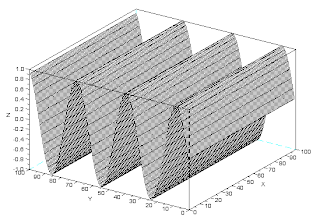
Figure 4. A sinusoid along x

z = sin(10*(X+1));mesh(z);

 Figure 5. A circular aperture with a gaussian transparency

gauss = exp(-((X*3).^2 + (Y*3).^2));
A(find(r<0.8)) = 1;
imshow(A*gauss);

Figure 6. A grating

A(find(sin(39*(Y+1)) <0 & -0.5<X & X<0.5))=1;imshow(A);

 For this experiment, I would give myself a grade of 10 for being able to satisfy the requirements. I'm excited to create more complicated shapes with mesh!